Lensing a flat-sky map

using CMBLensing, PythonPlot

    CondaPkg Found dependencies: /home/cosmo/.julia/packages/PythonCall/wXfah/CondaPkg.toml
    CondaPkg Found dependencies: /home/cosmo/.julia/packages/PythonPlot/KcWMF/CondaPkg.toml
    CondaPkg Found dependencies: /home/cosmo/CMBLensing/CondaPkg.toml
    CondaPkg Dependencies already up to date

First we load a simulated unlensed field, $f$, and lensing potential, $\phi$,

(;ds, f, ϕ) = load_sim(
    θpix  = 2,       # size of the pixels in arcmin
    Nside = 256,     # number of pixels per side in the map
    T     = Float32, # Float32 or Float64 (former is ~twice as fast)
    pol   = :I,      # :I for Intensity, :P for polarization, or :IP for both
);

We can lense the map with LenseFlow,

f̃ = LenseFlow(ϕ) * f;

And flip between lensed and unlensed maps,

animate([f,f̃], fps=1)

The difference between lensed and unlensed,

plot(f-f̃);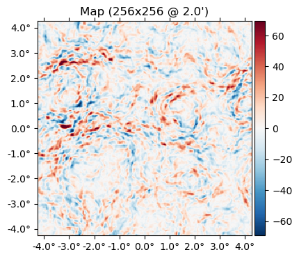

png

Loading your own data

CMBLensing flat-sky Field objects like f or ϕ are just thin wrappers around arrays. You can get the underlying data arrays for $I(\mathbf{x})$, $Q(\mathbf{x})$, and $U(\mathbf{x})$ with f[:Ix], f[:Qx], and f[:Ux] respectively, or the Fourier coefficients, $I(\mathbf{l})$, $Q(\mathbf{l})$, and $U(\mathbf{l})$ with f[:Il], f[:Ql], and f[:Ul],

mapdata = f[:Ix]

256×256 view(::Matrix{Float32}, :, :) with eltype Float32:
 -145.974  -134.078  -120.918   -104.631   …  -198.186   -189.465   -165.136
 -151.474  -135.045  -112.763    -82.849      -195.957   -189.838   -169.182
 -155.79   -132.561  -103.972    -71.0759     -191.606   -189.953   -174.786
 -163.767  -133.438   -97.1812   -64.4921     -181.429   -188.062   -182.345
 -170.502  -140.476  -102.696    -70.9361     -168.72    -185.25    -186.682
 -169.757  -138.253  -109.184    -85.781   …  -166.162   -190.397   -192.965
 -162.508  -128.104  -109.931    -98.6977     -180.037   -200.872   -195.384
 -146.524  -117.715  -108.818   -106.16       -197.524   -202.771   -182.602
 -129.488  -113.162  -112.093   -109.124      -200.593   -192.268   -161.24
 -122.481  -116.836  -118.426   -110.656      -191.381   -179.099   -148.322
 -130.762  -127.468  -128.24    -119.368   …  -188.151   -177.104   -152.178
 -150.812  -145.954  -144.624   -137.148      -195.465   -188.456   -170.024
 -177.295  -169.391  -162.297   -152.499      -207.631   -206.448   -192.582
    ⋮                                      ⋱                           ⋮
 -147.817  -162.499  -167.816   -165.661       -67.7319   -90.9288  -122.547
 -146.813  -167.485  -176.803   -173.321   …   -77.4413   -95.0936  -121.279
 -165.042  -182.129  -183.873   -174.909       -99.3494  -116.674   -141.429
 -179.04   -190.76   -189.502   -179.477      -115.868   -136.135   -159.87
 -176.421  -188.881  -194.36    -190.284      -120.681   -141.567   -162.437
 -170.162  -182.07   -192.207   -192.601      -125.044   -144.057   -158.927
 -162.916  -165.907  -172.879   -172.803   …  -144.07    -155.13    -159.96
 -154.837  -145.103  -148.443   -148.525      -174.634   -175.237   -166.964
 -155.639  -143.003  -147.58    -145.384      -201.79    -194.739   -176.193
 -161.363  -157.656  -164.607   -157.939      -213.942   -202.75    -180.083
 -157.673  -158.602  -163.825   -157.693      -210.279   -198.622   -173.913
 -147.652  -143.465  -141.517   -135.26    …  -202.147   -192.109   -166.505

If you have your own map data in an array you'd like to load into a CMBLensing Field object, you can construct it as follows:

FlatMap(mapdata, θpix=3)

65536-element 256×256-pixel 3.0′-resolution LambertMap{SubArray{Float32, 2, Matrix{Float32}, Tuple{Base.Slice{Base.OneTo{Int64}}, Base.Slice{Base.OneTo{Int64}}}, true}}:
 -145.97389
 -151.4739
 -155.79005
 -163.76654
 -170.50171
 -169.75746
 -162.50768
 -146.52411
 -129.48804
 -122.481
 -130.76152
 -150.81198
 -177.29526
    ⋮
 -122.54673
 -121.27854
 -141.42937
 -159.87007
 -162.43677
 -158.92677
 -159.95978
 -166.96414
 -176.19281
 -180.08272
 -173.91293
 -166.50537

For more info on Field objects, see Field Basics.

Inverse lensing

You can inverse lense a map with the \ operator (which does A \ b ≡ inv(A) * b):

LenseFlow(ϕ) \ f;

Note that this is true inverse lensing, rather than lensing by the negative deflection (which is often called "anti-lensing"). This means that lensing then inverse lensing a map should get us back the original map. Lets check that this is the case:

Ns = [7 10 20]
plot([f - (LenseFlow(ϕ,N) \ (LenseFlow(ϕ,N) * f)) for N in Ns],
    title=["ODE steps = $N" for N in Ns]);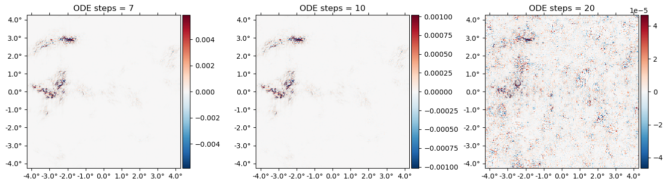

png

A cool feature of LenseFlow is that inverse lensing is trivially done by running the LenseFlow ODE in reverse. Note that as we crank up the number of ODE steps above, we recover the original map to higher and higher precision.

Other lensing algorithms

We can also lense via:

PowerLens: the standard Taylor series expansion to any order:

\[ f(x+\nabla x) \approx f(x) + (\nabla f)(\nabla \phi) + \frac{1}{2} (\nabla \nabla f) (\nabla \phi)^2 + ... \]

TayLens (Næss&Louis 2013): like PowerLens, but first a nearest-pixel permute step, then a Taylor expansion around the now-smaller residual displacement

plot([(PowerLens(ϕ,2)*f - f̃) (Taylens(ϕ,2)*f - f̃)], 
    title=["PowerLens - LenseFlow" "TayLens - LenseFlow"]);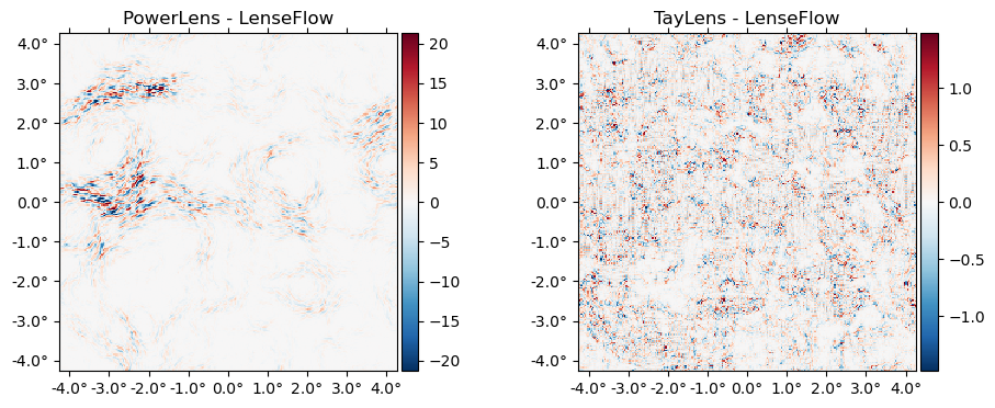

png

Benchmarking

LenseFlow is highly optimized code since it appears on the inner-most loop of our analysis algorithms. To benchmark LenseFlow, note that there is first a precomputation step, which caches some data in preparation for applying it to a field of a given type. This was done automatically when evaluating LenseFlow(ϕ) * f but we can benchmark it separately since in many cases this only needs to be done once for a given $\phi$, e.g. when Wiener filtering at fixed $\phi$,

using BenchmarkTools

@benchmark precompute!!(LenseFlow(ϕ),f)

BenchmarkTools.Trial: 492 samples with 1 evaluation.
 Range (min … max):   7.562 ms … 21.851 ms  ┊ GC (min … max):  0.00% … 13.12%
 Time  (median):     10.605 ms              ┊ GC (median):    26.57%
 Time  (mean ± σ):   10.154 ms ±  1.593 ms  ┊ GC (mean ± σ):  20.99% ± 11.49%

                                     ▄█▇▂                      
  ▅██▅▂▁▂▁▁▁▂▃▄▃▁▁▁▁▂▁▁▁▁▁▁▁▁▁▁▁▁▁▂▃▆████▆▃▂▂▂▄▅▇▅▃▂▁▂▁▁▁▁▁▁▂ ▃
  7.56 ms         Histogram: frequency by time        12.5 ms <

 Memory estimate: 62.99 MiB, allocs estimate: 804.

Once cached, it's faster and less memory intensive to repeatedly apply the operator:

@benchmark Lϕ * f setup=(Lϕ=precompute!!(LenseFlow(ϕ),f))

BenchmarkTools.Trial: 179 samples with 1 evaluation.
 Range (min … max):  15.763 ms … 30.315 ms  ┊ GC (min … max): 0.00% … 10.01%
 Time  (median):     16.241 ms              ┊ GC (median):    0.00%
 Time  (mean ± σ):   17.886 ms ±  2.931 ms  ┊ GC (mean ± σ):  3.21% ±  5.71%

  ▄█▇▃              ▃▁                     ▁                   
  ████▁█▄▁▄▁▆▁▄▁▁▄▁███▇▄▄▄▁▁▁▄▄▁▁▁▄▄▄▁▁▆▁▄▇██▆▁▁▁▁▁▁▁▁▁▁▁▄▄▁▆ ▄
  15.8 ms      Histogram: log(frequency) by time      26.5 ms <

 Memory estimate: 16.13 MiB, allocs estimate: 441.

Note that this documentation is generated on limited-performance cloud servers. Actual benchmarks are likely much faster locally or on a cluster, and yet (much) faster on GPU.